MnSi
This example will guide you through the experimental investigation conducted by Amato et al. and Dalmas de Réotier et. al reported in the following journal articles [Amato2014], [DalmasdeReotier2016].
For the complete code see run_example.py in the MnSi the examples directory of the muesr package (or open it on github).
Note
This is an advanced example. It is assumed that you already familiarized with Muesr by following one of the other examples or the tutorial.
Scientific background
MnSi has a cubic lattice structure with lattice constant 4.558 Å. It has P213 (No. 198) space group symmetry and the Mn-ion occupy the position (0.138,0.138,0.138), while the Si-ion the position (0.845,0.845,0.845).
At T ~ 0 K, the magnetic structure of MnSi is characterized by spins forming a left-handed incommensurate helix with a propagation vector k≃0.036 Å^−1 in the [111] direction [5–7]. The static Mn moments ( ∼0.4μB for T→0 K) point in a plane perpendicular to the propagation vector.
Dipolar Tensor
Given the number of oscillations that are found in the experiment, only a Wyckoff site of type 4a is possible. We therefore proceed by inspecting the dipolar tensor for all points the points of type 4a which happen to be in the 111 (and equivalent) direction of the cubic cell. As a first step, we will identify the number of parameters that characterize the dipolar tensor numerically by visually checking the dipolar tensor elements for all the equivalent sites. This can be done much more accurately analytically but a numerical check can come in handy.
37 38 39 40 41 42 43 44 45 46 47 48 49 50 51 52 53 54 55 56 57 58 59 60 61 62 63 64 65 66 67 68 69 70 71 72 73 74 75 76 77 78 79 | # this is a general position along the 111,
# just to identify the form of the dipolar tensor for the sites
# along the 111
s.add_muon([0.45,0.45,0.45])
# we find the remainig eq muon sites
muon_find_equiv(s)
# apply an arbitrary small field to select magnetic atoms.
# the abslute value is not used, but it must be different from 0.
APP_FCs = 0.001*np.array([[0,0,1],
[0,0,1],
[0,0,1],
[0,0,1],
[0,0,0],
[0,0,0],
[0,0,0],
[0,0,0]], dtype=np.complex)
s.new_mm()
s.mm.desc = "Applied field"
s.mm.k = np.array([0,0,0])
s.mm.fc = APP_FCs
# Calculate the dipolar tensor. Result is in Ang^-3
dts = dipten(s, [30,30,30],50) # supercell size set to 30 unit cells,
# a 50 Ang sphere si certainly contained.
# Print the muon site for all the 4 equivalent site.
for i, pos in enumerate(s.muons):
print(("\nFrac. muon position: {:2.3f} {:2.3f} {:2.3f}\n" + \
"Dipolar Tensor: {:2.3f} {:2.3f} {:2.3f}\n" + \
" {:2.3f} {:2.3f} {:2.3f}\n" + \
" {:2.3f} {:2.3f} {:2.3f}\n").format( \
*(pos.tolist() + (dts[i] * 6.022E24/1E24/4).flatten().tolist()) \
)
)
# We will now identify the position of the muon site using the TF data
# remove all defined positions for the search
muon_reset(s)
|
In line 40 we add one of the four symmetry equivalent positions for a muon in the 4a Wyckoff site and we let the code find the other sites in line 42 with the function muon_find_equiv. In line 46 we define arbitrary small Fourier components which are used to specify which atoms are magnetic (Mn in this case). We finally add this sort of magnetic order to the sample description in lines 56-59 The value of the propagation vector given in line 58 can be omitted (resulting in 0 as default )as it is not used anywhere in this initial estimation of the dipolar tensor. The non-zero values of the dipolar tensor, shown at standard output, are
Frac. muon position: 0.450 0.450 0.450
Dipolar Tensor: 0.000 0.092 0.092
                0.092 0.000 0.092
                0.092 0.092 0.000


Frac. muon position: 0.050 0.550 0.950
Dipolar Tensor: 0.000 0.092 -0.092
                0.092 -0.000 -0.092
                -0.092 -0.092 0.000


Frac. muon position: 0.550 0.950 0.050
Dipolar Tensor: -0.000 -0.092 0.092
                -0.092 0.000 -0.092
                0.092 -0.092 0.000


Frac. muon position: 0.950 0.050 0.550
Dipolar Tensor: 0.000 -0.092 -0.092
                -0.092 0.000 0.092
                -0.092 0.092 -0.000
In order to compare with the experiment, we will evaluate the dipolar tensor for 100 values along the 111 direction.
84 85 86 87 88 89 90 91 92 93 94 95 96 97 98 | positions = np.linspace(0,1,100)
for pos in positions:
s.add_muon([pos,pos,pos])
dts = dipten(s, [30,30,30],50) # supercell size set to 30 unit cells,
# a 50 Ang sphere si certainly contained.
values_for_plot = np.zeros_like(positions)
for i, dt in enumerate(dts):
# to reproduce the plot of Amato et. al, we convert to emu/mol
values_for_plot[i] = dt[0,1] * 6.022E24/1E24/4 # (cm^3/angstrom^3) = 1E24
# remove all defined positions for the search
muon_reset(s)
|
Lines 99-110 produce the following figure:
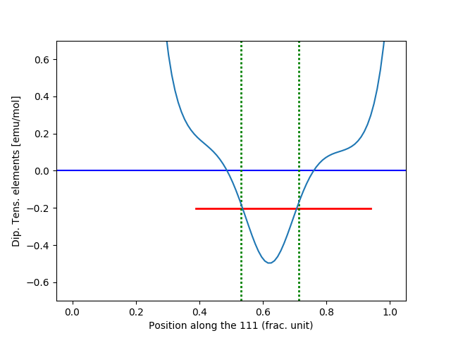
which is essentially what is reported in [Amato2014].
Local Fields
In order to calculate the local fields at the muon site in the helical state, we will first define the magnetic order and then evaluate the local fields with a optimized algorithm for incommensurate magnetic structures.
Let us first create a few useful variables for the definition of the Fourier components (FC).
116 117 118 119 120 121 122 123 124 125 126 127 128 129 130 131 132 133 134 135 136 137 138 139 140 141 142 143 144 145 146 147 | scaled_pos = s.cell.get_scaled_positions()
pos_Mn1 = scaled_pos[0]
pos_Mn2 = scaled_pos[1]
pos_Mn3 = scaled_pos[2]
pos_Mn4 = scaled_pos[3]
# let's do some simple math
a = 4.558 # Ang
a_star = 2*np.pi/a #Ang^-1
norm_k = 0.035 # Å −1
k_astar = k_bstar = k_cstar = (1/np.sqrt(3))*norm_k
k_rlu = np.array([k_astar,k_bstar,k_cstar])/a_star # this only works for a cubic lattic
# rotation plane must be perpendicular to k // [111]
# let's chose one direction to be in the [1,-1,0] direction and find the other
def uv(vec):
return vec/np.linalg.norm(vec)
k_u = uv(k_rlu) # unitary vector in k direction
a = uv([1,-1,0]) # one of the two directions which define the plane of
# the rotation
b = np.cross(k_u,a) # the other vector (perp. to a) defining the plane
# where the moments lie.
# There are two choices here: left handed or right
# handed spiral. We will do both.
|
We can now define both a left handed and a right handed helix.
151 152 153 154 155 156 157 158 159 160 161 162 163 164 165 166 167 168 169 170 171 |
# assuming that, at x=0, a Mn moment is // a, the spiral can be obtained as
RH_FCs = 0.385 * np.array([(a+1j*b)*np.exp(-2*np.pi*1j*np.dot(k_rlu,pos_Mn1)),
                         (a+1j*b)*np.exp(-2*np.pi*1j*np.dot(k_rlu,pos_Mn2)),
                         (a+1j*b)*np.exp(-2*np.pi*1j*np.dot(k_rlu,pos_Mn3)),
                         (a+1j*b)*np.exp(-2*np.pi*1j*np.dot(k_rlu,pos_Mn4)),
                         [0,0,0],
                         [0,0,0],
                         [0,0,0],
                         [0,0,0]
                        ])
# Notice the minus sign.
LH_FCs = 0.385 * np.array([(a-1j*b)*np.exp(-2*np.pi*1j*np.dot(k_rlu,pos_Mn1)),
                         (a-1j*b)*np.exp(-2*np.pi*1j*np.dot(k_rlu,pos_Mn2)),
                         (a-1j*b)*np.exp(-2*np.pi*1j*np.dot(k_rlu,pos_Mn3)),
                         (a-1j*b)*np.exp(-2*np.pi*1j*np.dot(k_rlu,pos_Mn4)),
                         [0,0,0],
                         [0,0,0],
                         [0,0,0],
                         [0,0,0]
                        ])
|
We finally add the muon positions and the two magnetic orders with the commands
177 178 179 180 181 182 183 184 185 186 187 188 189 190 | s.new_mm()
s.mm.desc = "Right handed spiral"
s.mm.k = k_rlu
s.mm.fc = RH_FCs
s.new_mm()
s.mm.desc = "Left handed spiral"
s.mm.k = k_rlu
s.mm.fc = LH_FCs
s.add_muon([0.532, 0.532, 0.532])
muon_find_equiv(s)
|
Note
When a new magnetic order is added, the index is automatically incremented and the new entry is immediately selected
In order to get the local contributions to the magnetic field at the muon site we use the function locfield function and specify the ‘i’ sum type.
192 193 194 195 196 197 | # For Reft Handed
s.current_mm_idx = 1; # N.B.: indexes start from 0 but idx=0 is the transverse field!
r_RH = locfield(s, 'i',[50,50,50],100,nnn=3,nangles=360)
s.current_mm_idx = 2;
r_LH = locfield(s, 'i',[50,50,50],100,nnn=3,nangles=360)
|
By default, the contact coupling is 0 for all sites. In order to have a contact term different from 0 we have to set the parameter ACont for all the muon sites that we defined.
200 201 202 | for i in range(4):
r_RH[i].ACont = ContatExp
r_LH[i].ACont = ContatExp
|
The lines 205-2624produce the following pictures:
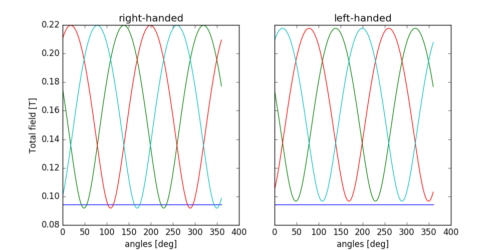
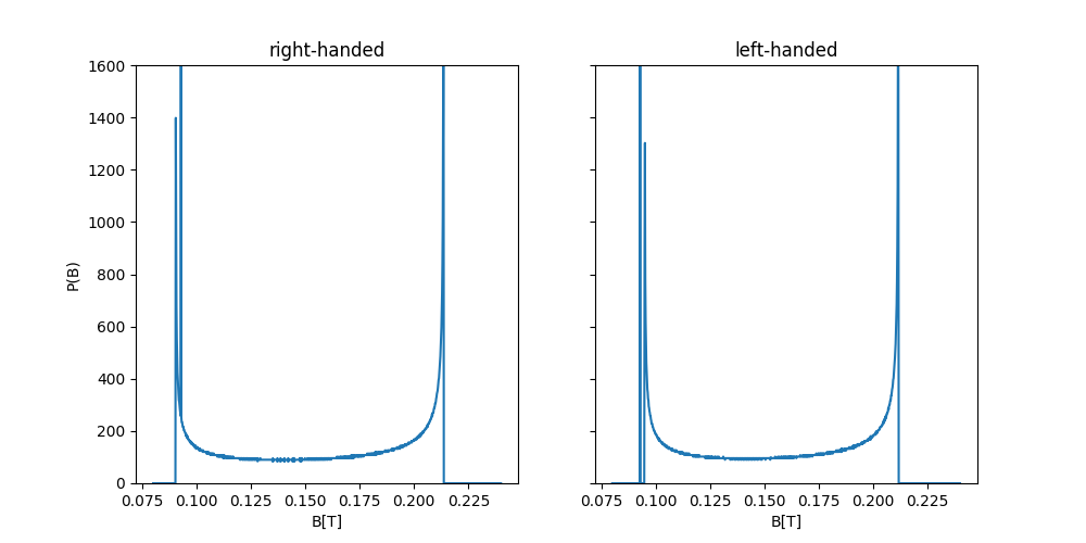
Interestingly, left-handed and right-handed orders produce different local field. This is due to the lack of inversion symmetry.
The phase between Mn atoms in the unit cell
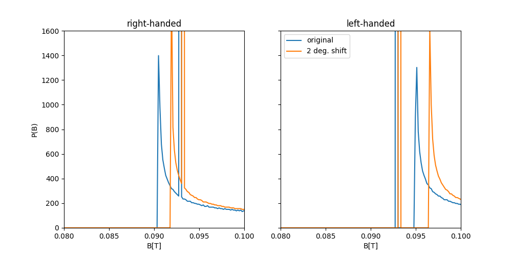
Dalmas De and Reotier colleagues pointed out that the complete description of the spiral phase requires three additional degrees of freedom: the two angles describing the misalignmente between the rotation plane of the Mn moments and the plane perpendicular to the propagation vector \(k\) and the phase between the helices in the Mn sites belonging to the two crystallographic orbits (see [DalmasdeReotier2016]). This last parameter strongly influence the results.
Here we define a phase shift of \(\phi=2\) degrees as reported in the article mentioned above.
293 294 295 296 297 298 299 300 301 302 303 304 305 306 307 308 309 310 311 | RH_FCs = 0.385 * np.array([(a+1j*b)*np.exp(-2*np.pi*1j*np.dot(k_rlu,pos_Mn1)-np.pi*2./180.),
(a+1j*b)*np.exp(-2*np.pi*1j*np.dot(k_rlu,pos_Mn2)),
(a+1j*b)*np.exp(-2*np.pi*1j*np.dot(k_rlu,pos_Mn3)),
(a+1j*b)*np.exp(-2*np.pi*1j*np.dot(k_rlu,pos_Mn4)),
[0,0,0],
[0,0,0],
[0,0,0],
[0,0,0]
])
# Notice the minus sign.
LH_FCs = 0.385 * np.array([(a-1j*b)*np.exp(-2*np.pi*1j*np.dot(k_rlu,pos_Mn1)-np.pi*2./180.),
(a-1j*b)*np.exp(-2*np.pi*1j*np.dot(k_rlu,pos_Mn2)),
(a-1j*b)*np.exp(-2*np.pi*1j*np.dot(k_rlu,pos_Mn3)),
(a-1j*b)*np.exp(-2*np.pi*1j*np.dot(k_rlu,pos_Mn4)),
[0,0,0],
[0,0,0],
[0,0,0],
[0,0,0]
])
|
Repeating the same procedure discussed above leads to the following comparison between the magnetic structures with \(\phi=0\) (blue) and and \(\phi=2\) deg (orange).