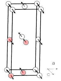
La2CuO4

Another antiferromagnetic insulator with a slightly more complicated unit cell

import numpy as np
from muesr.engines.clfc import locfield
from muesr.core import Sample
from muesr.engines.clfc import find_largest_sphere
from muesr.i_o import load_cif
from muesr.utilities import mago_add, show_structure # mago_add is a helper to add magnetic structures
np.set_printoptions(suppress=True,precision=4)

         Spg Library not loaded

Start again by creating a sample, loading a cif into it and adding a tentative muon site

la2cuo4 = Sample()
load_cif(la2cuo4,"/home/roberto.derenzi/tex/mytalks/ISIS-19-03-2018/dipolar_examples/La2CuO4_Cmca_new.cif")

la2cuo4.add_muon([-0.14, 0.1770, -0.1740]) # 1.07 A from apical O

Cmca group 64, 28 atoms: 8 non magnetic La, 4 magnetic Cu, 16 non magnetic O.

Magnetic structure from Vaknin et al. PRL 58 2802, Cu moment is 0.6 Bohr magnetons, i.e. 1 µB with quantum S=1/2 spin reduction in 2D, see e.g. T.Ishikawa and T.Oguchi, Prog. Th. Phys. 54 1282 (1975)

First do it the long way, as in the CoF2 case

la2cuo4.new_mm() # magnetic structure from Vaknin et al PRL 58 2802
# insert the k vector, in a pseudo-ferromagnetic cell, with a base
la2cuo4.mm.k=np.array([0.0,0.0,0.0])
# insert the m_nu,k fourier components for each atom according to CIF
la2cuo4.mm.fc= np.array([[0.0+0.j, 0.0+0.j, 0.0+0.j],[0.0+0.j, 0.0+0.j, 0.0+0.j],
                    [0.0+0.j, 0.0+0.j, 0.0+0.j],[0.0+0.j, 0.0+0.j, 0.0+0.j],
                    [0.0+0.j, 0.0+0.j, 0.0+0.j],[0.0+0.j, 0.0+0.j, 0.0+0.j],
                    [0.0+0.j, 0.0+0.j, 0.0+0.j],[0.0+0.j, 0.0+0.j, 0.0+0.j],
                    [0.0+0.j, 0.0+0.j, 0.6+0.j],[0.0+0.j, 0.0+0.j, 0.6+0.j], # magnetic Cu
                    [0.0+0.j, 0.0+0.j, -0.6+0.j],[0.0+0.j, 0.0+0.j, -0.6+0.j], # magnetic Cu
                    [0.0+0.j, 0.0+0.j, 0.0+0.j],[0.0+0.j, 0.0+0.j, 0.0+0.j],
                    [0.0+0.j, 0.0+0.j, 0.0+0.j],[0.0+0.j, 0.0+0.j, 0.0+0.j],
                    [0.0+0.j, 0.0+0.j, 0.0+0.j],[0.0+0.j, 0.0+0.j, 0.0+0.j],
                    [0.0+0.j, 0.0+0.j, 0.0+0.j],[0.0+0.j, 0.0+0.j, 0.0+0.j],
                    [0.0+0.j, 0.0+0.j, 0.0+0.j],[0.0+0.j, 0.0+0.j, 0.0+0.j],
                    [0.0+0.j, 0.0+0.j, 0.0+0.j],[0.0+0.j, 0.0+0.j, 0.0+0.j],
                    [0.0+0.j, 0.0+0.j, 0.0+0.j],[0.0+0.j, 0.0+0.j, 0.0+0.j],
                    [0.0+0.j, 0.0+0.j, 0.0+0.j],[0.0+0.j, 0.0+0.j, 0.0+0.j]])
la2cuo4.mm.desc = 'stripe along b with k = 0'

La2CuO4 Cmca setting according to Vaknin PRL 58 2802

title

show_structure(la2cuo4,visualizationTool='V')

True

radius=find_largest_sphere(la2cuo4,[100, 100, 100])
r=locfield(la2cuo4, 's', [100, 100, 100] ,radius)
print('vector B_dip components = {} T, B_dip = {:.4} T'.format(r[0].D,np.linalg.norm(r[0].D,axis=0)))
# save_sample(la2cuo4,'La2CuO4-stripe-as-fm.yaml')

vector B_dip components = [ 0.0035 -0.039  -0.0131] T, B_dip = 0.04128 T

compare the above result with the experimental value Bexp = 0.041 T from Budnick et al., Phys Lett A 124, 103